Classifiable Graph Attributes
The hm software is able to apply each of the classifiers to each of the
17 classifiable graph attributes listed below. The attributes
vary by their visual saliency and by the number of states they are able to
express. Fill color, color, and shape (including the polygon attributes) are
most salient for nodes, followed by font color, pen width, and style. Color,
style, and arrowhead are most salient for edges, followed by font size,
font color, and pen width.
(show-classifiable-attributes)
edge-color-by
edge-style-by
node-color-by
node-shape-by
node-style-by
edge-fontsize-by
edge-penwidth-by
node-penwidth-by
edge-arrowhead-by
edge-fontcolor-by
node-fillcolor-by
node-fontcolor-by
node-polygon-skew-by
node-polygon-image-by
node-polygon-sides-by
node-polygon-distortion-by
node-polygon-orientation-by
Colors
The hm software offers several color palettes that might be useful in
different situations. However, color should be handled with care because it is
easy to misuse it.
Edward Tufte’s chapter on “Color and Information” in the book Envisioning Information starts off like this:
In representing and communicating information, how are we to benefit from color’s great dominion? Human eyes are exquisitely sensitive to color variations: a trained colorist can distinguish among 1,000,000 colors, at least when tested under contrived conditions of pairwise comparison. Some 20,000 colors are accessible to many viewers, with the constraints for practical applications set by the early limits of human visual memory rather than the capacity to discriminate locally between adjacent tints. For encoding abstract information, however, more than 20 or 30 colors frequently produce not diminishing but negative returns.
Tying color to information is as elementary and straightforward as color technique in art, “To paint well is simply this: to put the right color in the right place,” in Paul Klee’s ironic prescription. The often scant benefits derived from coloring data indicate that even putting a good color in place is a complex matter. Indeed, so difficult and subtle that avoiding catastrophe becomes the first principle in bringing color to information: Above all, do no harm.
With this in mind, the hm software uses a selection of named and indexed color
palettes.
Named Color Palettes
Colors from named color palettes are indicated by a color name, such as
burlywood3, coral1, or darkgoldenrod. Named color palettes are useful in
situations where you know ahead of time how many colors will be needed, or when
you have need or desire to use particular hues. However, choosing colors that
work well with one another is difficult for many people and, as Tufte reminds us,
catastrophe is a real possibility.
The three named color palettes used by hm software include the two general
purpose palettes, X11 and SVG, and the designer palette, Solarized.
X11
The hm software recognizes 782 X11 color names, which generally correspond to
the Graphviz dot X11 color names. By far the most useful of these are white
and black, with dimgray (or dimgrey), gray (or grey), and lightgray
(or lightgrey) often coming in handy.
SVG
The SVG palette has 147 names for somewhat fewer colors, given that some colors
have multiple names. In general, this is a subset of the X11 colors that is most
useful when graphics output will be scalar vector graphics. The Graphviz dot SVG
color names are supported by the hm software.
Solarized
The Solarized color palette was developed by a designer interested in computer
graphics. It includes two sets of background tones, a set of four tones for
content, and eight accent colors. The accent colors are suited for categorical
variables and might be useful for classifications with relatively few
distinctions such as units, adjacent, and reachable. In some cases, they
might be useful for periods or phases.
A notable feature of the Solarized palette is the relative ease of switching from a color scheme with a dark background to one with a light background (Fig. 1). A characteristic of the Solarized palette is accent colors—in this case violet, cyan, and orange—look good on either a dark or light background. An example project is included to show off this property of the Solarized palette.
When the following command is run on a Linux system, the graph in Figure 1 results.
(run-project/example :roskams-h-solarized-light)
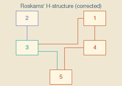
Figure 1: A correct Harris matrix for Figure classified by adjacency to Context 2. Colors are from the Solarized light palette.
There is an informative website that describes Ethan Schoonover’s Solarized colors.
Indexed Color Palettes
Colors in indexed color palettes are identified by numbers, rather than names. This makes them easy to use in situations where the number of colors needed is not known ahead of time. In addition, the color palettes have been designed to include colors that work well together, so graphs that use them can have a polished look that might be difficult to achieve otherwise.
There are three kinds of indexed color palette that are useful for different kinds of data:
- sequential
- colors move from dark to light along a single “path” through color space, which makes it easy to visualize the magnitude of a value
- diverging
- colors move from dark to light and back to dark again as they move from one edge of the rainbow to the other, a pattern that highlights the middle color and is useful for data that have both location and scale
- qualitative
- colors are chosen to be distinct from one another, without giving emphasis to one or another, which is useful for categorical data
The hm software uses a color index that is 0 based for all of the indexed
color palettes. Note that this is different than the usual scheme for the
Brewer color palettes in which the base color is 1.
The hm software offers two sets of indexed color palettes, one developed by
the ColorBrewer project, and another developed at the Center for Exploration
Targeting.
Brewer Color Palettes
The Brewer color palettes are built into the GraphViz dot software. There are
several families of 3 to 12 color palettes, which are most useful for the simple
classifications. The hm software accepts the family name of the color scheme
and then chooses which palette to use based on the number of colors needed. So,
for example, the hm software user might choose accent, blues, or brbg
and the software might apply accent3, blues7, or brbg 5, as appropriate.
Note that the paired palette is useful for classifications such as adjacent
and reachable that yield three values. In these cases, the origin and
adjacent or reachable nodes can be colored with the same hue, and non-adjacent
or unreachable nodes can be colored with a different hue. Figure
illustrates use of the paired color palette with a
reachable classification.
Center for Exploration Targeting Color Palettes
These are 256 color palettes that were designed to be “perceptually uniform”, which means that none of the colors sticks out from the others. The idea behind perceptual uniformity of colors in the palette is that perceptual variation in a graphic that uses these color palettes will primarily track variation in the underlying data.
These color palettes will be most useful for the levels and distance
classifications, which might require dozens of distinct colors to represent the
range of values. Because both of these classifications yields a number important
for its magnitude, the palettes included with the hm software are mostly
sequential (or linear), but also include a rainbow palette.
The name of the palette used by the hm software is shown in the first column
of Table 1. The second column gives the name of the color file
distributed by Colorcet; the names of these files are based on the palette
labels displayed at the Colorcet website.
| name | file |
|---|---|
| cet-bgyw | linear_bgyw_15-100_c67_n256.csv |
| cet-kbc | linear_blue_5-95_c73_n256.csv |
| cet-blues | linear_blue_95-50_c20_n256.csv |
| cet-bmw | linear_bmw_5-95_c86_n256.csv |
| cet-inferno | linear_bmy_10-95_c71_n256.csv |
| cet-kgy | linear_green_5-95_c69_n256.csv |
| cet-gray | linear_grey_0-100_c0_n256.csv |
| cet-dimgray | linear_grey_10-95_c0_n256.csv |
| cet-fire | linear_kryw_0-100_c71_n256.csv |
| cet-kb | linear_ternary-blue_0-44_c57_n256.csv |
| cet-kg | linear_ternary-green_0-46_c42_n256.csv |
| cet-kr | linear_ternary-red_0-50_c52_n256.csv |
| cet-rainbow | rainbow_bgyr_35-85_c72_n256.csv |
Nodes
The dot software provides many ways to control how nodes are displayed.
Shapes
Node shapes can be set individually, or they can be assigned by hm based on
the value of a classifier. The names of the shapes are taken from the dot software.
Here is an example of node shapes set individually in the configuration file.
[Graphviz sequence reachability node shapes]
origin = box
reachable = triangle
not-reachable = oval
In situations where it is not possible to specify node shapes individually, the
hm software uses a lookup table to map a classifier to a node shape. The
lookup table can be displayed with the following function call.
(show-map :node-shape)
0 --> box
1 --> trapezium
2 --> ellipse
3 --> egg
4 --> triangle
5 --> diamond
6 --> oval
7 --> circle
8 --> house
9 --> pentagon
10 --> parallelogram
11 --> square
12 --> star
13 --> hexagon
14 --> septagon
15 --> octagon
16 --> doublecircle
17 --> doubleoctagon
18 --> tripleoctagon
19 --> invtriangle
20 --> invtrapezium
21 --> invhouse
22 --> Mdiamond
23 --> Msquare
24 --> Mcircle
25 --> lpromoter
26 --> larrow
27 --> underline
28 --> note
29 --> tab
30 --> folder
31 --> box3d
32 --> component
33 --> cds
34 --> signature
35 --> rpromoter
36 --> rarrow
Polygons
Polygons offer another way to classify node shapes. Instead of working with a
fixed number of shapes, polygons can take on almost any shape, varying
continuously along dimensions defined by skew, sides, distortion, and
orientation. It is even possible to associate images with polygons.
In theory, the various dimensions of a polygon might be associated with different classifiers, with each combination of classifier values yielding its own distinct polygon. The key here is, of course, the term “distinct”. At some point, complexity in the underlying data defeats the graphical purpose, yielding a complex graphic that defies interpretation.
Figure 2 shows an example of polygons in use, which builds on the classification of Harris’ Figure 12 by periods (see fig. ).
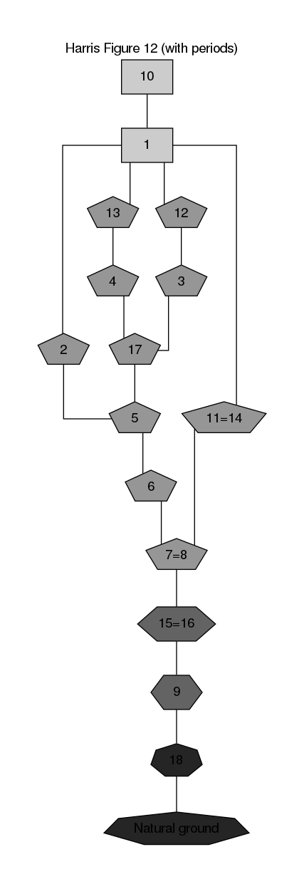
Figure 2: Stratigraphic DAG for the information on Figure and periodized according to Figure . Note that the number of node sides and node fill color both reflect the periods classification.
Figure 2 can be produced on a Linux system with the following function call:
(run-project/example :fig-12-polygon)
Polygons require a bit of set up in the configuration file. The node-shape-by
option must be empty, node-shape must be set to polygon, and one of the
node-polygon-*-by attributes must be set to an appropriate classifier.
The configuration file for Figure 2 illustrates these points. The
options polygon-sides-min and polygon-sides-max set boundaries for the
allowable number of sides, while polygon-sides sets the shape of the base
polygon. So, in Figure 2 the latest period is shown as a rectangle
and each preceding period adds another side to the polygon.
[Graphviz sequence classification]
node-fillcolor-by = periods
node-fontcolor-by =
node-shape-by =
node-color-by =
node-penwidth-by =
node-style-by =
node-polygon-distortion-by =
node-polygon-image-by =
node-polygon-orientation-by =
node-polygon-sides-by = periods
...

[Graphviz sequence node attributes]
shape = polygon
...
polygon-sides = 4
polygon-sides-min = 3
polygon-sides-max = 16
Styles
Node styles can be set individually, or they can be assigned by hm based on
the value of a classifier. The names of the styles are taken from the dot
software. Note that some styles have to do with the node outline and others
have to do with the node fill. It is possible to set an option to two values,
one to control the node outline and the other to control the node fill.
Here is an example of node styles set individually in the configuration file. In each case, the first value controls the node outline and the second value controls the node fill.
[Graphviz sequence reachability node styles]
origin = solid,filled
reachable = dashed,filled
not-reachable = dotted,filled
In situations where it is not possible to specify the node styles individually,
the hm software uses a lookup table to map a classifier to a node style. The
lookup table can be displayed with the following function call.
(show-map :node-style)
0 --> solid
1 --> dashed
2 --> dotted
3 --> bold
4 --> rounded
5 --> diagonals
6 --> filled
7 --> striped
8 --> wedged
Arcs
The dot software provides several arc (or edge) styles and a wide range of
arrowheads.
Styles
The edge styles recognized by the hm software can be shown with the following
function call. In each case, the name used by hm matches the name used by dot.
(show-map :edge-style)
0 --> solid
1 --> dashed
2 --> dotted
3 --> bold
Arrowheads
The arrowhead styles recognized by the hm software can be shown with the
following function call. In each case, the name used by hm matches the name
used by dot.
(show-map :arrow-shape)
0 --> none
1 --> box
2 --> lbox
3 --> rbox
4 --> obox
5 --> olbox
6 --> orbox
7 --> crow
8 --> lcrow
9 --> rcrow
10 --> diamond
11 --> ldiamond
12 --> rdiamond
13 --> odiamond
14 --> oldiamond
15 --> ordiamond
16 --> dot
17 --> odot
18 --> inv
19 --> linv
20 --> rinv
21 --> oinv
22 --> olinv
23 --> orinv
24 --> normal
25 --> lnormal
26 --> rnormal
27 --> onormal
28 --> olnormal
29 --> ornormal
30 --> tee
31 --> ltee
32 --> rtee
33 --> vee
34 --> lvee
35 --> rvee
36 --> curve
37 --> lcurve
38 --> rcurve
39 --> icurve
40 --> licurve
41 --> ricurve